Ask a Climate Expert: How do I use netCDF files?

When downloading data from ClimateData.ca, users may encounter the option to download files in a format called “netCDF.” For those new to working with climate data, this file format might be unfamiliar. This article provides an overview of netCDF files, explaining their structure, why they are widely used, and offering tips on how to open them and read them.

What is a netCDF file?

Unlike a typical spreadsheet, which has just two dimensions, rows and columns, a Network Common Data Form, or netCDF file, can store data across any number of space and time dimensions. These files also contain other information about the data, like units and copyright information. Users can recognize a netCDF file by its “.nc” file extension. Every day, more climate data is being shared in netCDF format because it is flexible and standardized.

Understanding the power of netCDF files

NetCDF files are commonly used to store and access multi-dimensional gridded data. Imagine the Earth wrapped in a fine mesh, creating thousands of small boxes called grid cells across its surface. Each grid cell represents a specific area, typically defined by latitude and longitude. The values in a netCDF file denote a specific climate metric, such as temperature or precipitation, for each grid cell and at a specific time interval (i.e. daily, monthly, or annual).

Like a loaf of bread, it is possible to write a computer program that extracts a ‘slice’ of data across a specific space-time dimension within a netCDF file to examine how variables like temperature or precipitation change over time and space. This slice of data can then be mapped (a single slice of time over a wide area) or graphed on a time-series plot (a single location slice over a range of time). The netCDF file format accommodates both types of analyses.

Structure and components of a netCDF file

Figure 1 shows the key components of a netCDF file. The Dataset contains multiple DataArrays, which hold the actual data, such as variables like temperature and precipitation. These variables are structured along coordinates—in this case, latitude and longitude—and mapped across different dimensions (e.g., x, y, and t for time). The Dimensions represent the axes of the data (spatial and temporal), and Indexes provide reference points within these dimensions. This structure allows for efficient storage and access to large, multi-dimensional climate datasets. Each of these components is discussed in more detail below.

Figure 1. Visualization of the components of a netCDF file. Source: Data Structures (xarray.dev).
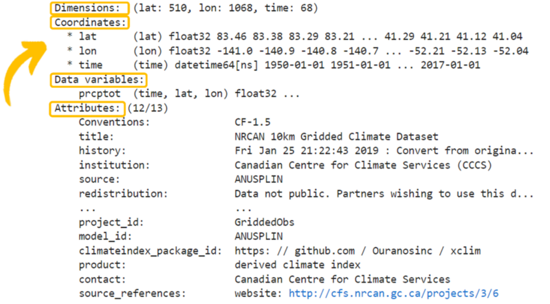
  • Dimensions/indexes: A dataset’s dimensions (or indexes) dictate its size and structure (e.g., the number of longitude/latitude points and the number of time steps). The most common dimensions in netCDF files that contain climate data are latitude, longitude, and time, but some datasets include other parameters such as elevation. For example, Figure 2 shows the dimensions of an NRCANMET netCDF file. The dimensions of this data file are 510 steps of lat (latitude), 1068 steps of lon (longitude), and 68 time steps.
  • Coordinates: Data coordinates indicate the exact location for each grid cell along each dimension (e.g., specific time, latitude, longitude). In Figure 2, you can see lists of values associated with each dimension (lat, lon, time). This shows us that the file covers latitudes from 83.46 to 41.04, longitudes from -141.0 to -52.04, and monthly time periods from January 1950 to January 2017.
  • Attributes: Details about the dataset are stored in the attributes, often including a basic description of the dataset, such as the model(s) used to produce the data and the production date. The attributes for the NRCANMET file in Figure 2 include information like the title, when the file was created or updated (history), and references for the data (source_references).
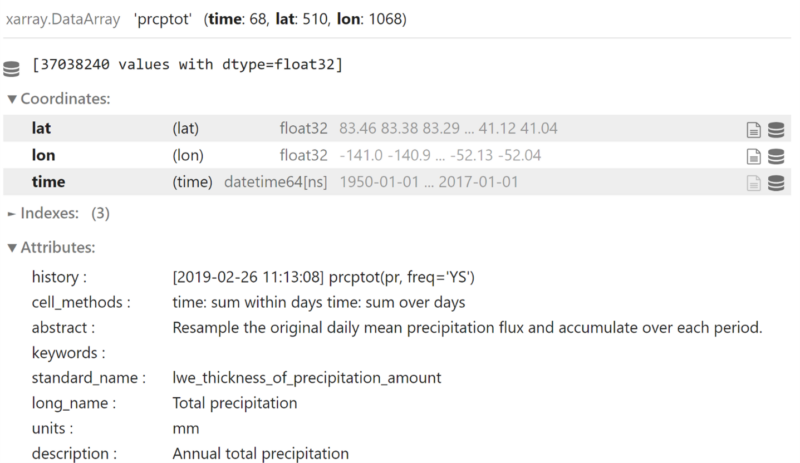
  • Data variables: This is where the climate data is stored. Each variable is situated within the same structure as the dimensions. For example, in our file in Figure 2, there is one data variable called prcptot, representing total precipitation, where each value has a latitude, longitude, and time dimension associated with it. One netCDF file can contain many variables, and each variable should have its own attributes as well, generally including a longer, more descriptive name for the variable and information about its units.
Figure 2. Description of the components of a NRCANMET precipitation netCDF file.

Why are netCDF files so widely used for climate data?

The ability of netCDF files to store multiple variables is only part of the reason for their growing popularity. Rather than needing separate files for metadata (information about the data stored), properly formatted netCDF files include attribute information such as data descriptions and units. This allows all necessary information to be contained within a single file, making it easier to use and share.

NetCDF files are typically smaller in size compared to other formats that store the same amount of data, as they compress well, saving storage space and facilitating sharing. One key reason for this efficiency is that coordinates, such as latitudes, longitudes, and time steps, are stored only once in the file, rather than being repeated for each data point. While netCDF files can still be large, most of the space is occupied by the actual climate data, unlike other formats such as comma-separated values (CSVs), where metadata and coordinates often take up more space. More benefits of netCDF files can be found in Unidata’s netCDF factsheet.

Opening and reading netCDF files

The main drawback of using netCDF files over other data formats, such as CSVs, is that they cannot be easily opened in spreadsheet programs like Microsoft Excel without installing add-ons. Instead, netCDF files are best suited for working within programming environments, such as Python or R. That said, there are some options for opening and viewing the contents of a netCDF file without needing to learn a programming language.

NASA’s Panoply NetCDF Data Viewer is a freely available tool used to view netCDF data. Within Panoply, users can generate simple figures and view different data slices. A Panoply walkthrough for beginners is available here. Note that Panoply requires Java, which is a paid software when used for commercial purposes (some free substitutes are available, which can be found in the Panoply readme file). For simple analysis, free plugins for Microsoft Excel allow for opening netCDF files, or data can be imported as a raster layer in GIS software like ArcGIS.

For those who have some computer programming experience, there are several coding libraries available that make working with netCDF files relatively straight-forward. One example is xarray, a netCDF library for Python users. Detailed tutorials for and examples of working with netCDF files using Python can be found on the PAVICS tutorial page, Pangeo Library, and xarray’s tutorials and videos page.

PAVICS (Power Analytics and Visualization for Climate Science) is a virtual, python-based, Jupyter notebook programming environment with xarray pre-installed. Users can create a login for PAVICS by visiting the site linked above.

The following code blocks demonstrate how to open and read a netCDF file within a Python programming environment like PAVICS. Users looking for more examples should consult the brief tutorial on PAVICS.


# Load the xarray package into python
import xarray as xr


# Specify the location of your netCDF data file
path = "path/to/file.nc"


# Import the file
ds = xr.open_dataset(path)

Note: netCDF files can take a long time to open compared to other file types, such as CSVs.

Typing the following command will print out a detailed list the netCDF file’s components (the same components detailed in Figure 2):


print(ds)

Similarly, here are some additional commands that users can use to view specific components of the file:

  • Look at a list of the dataset attributes: attrs
  • Look at dataset coordinates: coords
  • Look at a list of data variables (with their attributes): variables
  • For a simple list of data variable and coordinate names (without attributes): list(ds.variables)

Similarly, the following command will print out information about a specific variable within the netCDF file:


# Specify the variable of interest
var = "prcptot" # total precipitation in NRCANMET


print(ds[var])

Full Tutorial

After opening and viewing the contents of a netCDF file, users will very likely want to perform additional custom analyses (e.g. computing a custom metric, such as “number of days per year that are above 33 °C relative across a specific region”) prior to creating custom data visualizations (i.e. maps, graphs, and tables).

Again, PAVICS contains several built-in tutorials that showcase how to program these types of analyses and visualization commands. It is outside the scope of this article to explain how to develop these types of programs; however, the following code example demonstrates how one might approach this type of custom analysis.

The code block pasted below extracts and analyzes climate data from a netCDF file for a specific region, in this case, Terra Nova National Park. It begins by loading a shapefile that contains the boundary of the park and reprojects it to a standard geographic coordinate system. The program then accesses a climate dataset (specifically maximum temperature projections from one downscaled global climate model) from a specified URL and subsets the data to match the park’s geographical boundaries. Using the xclim library, it calculates the number of days per year where the maximum temperature exceeds 33°C. The program further computes two types of averages: one that averages the data spatially across the park, and another that averages the data temporally over the period from 2051 to 2080. Finally, it visualizes the data on a geographic map using a quadmesh plot, which includes a color scale to represent the results and a basemap for geographical context.


# Import necessary libraries
from xclim import atmos  # Climate indices calculations
from clisops.core import subset  # Subsetting and other operations on climate datasets
import xarray as xr  # For handling and analyzing multidimensional arrays (e.g., NetCDF files)
import geopandas as gpd  # For working with geospatial data
import pandas as pd  # Data manipulation and analysis
import matplotlib.pyplot as plt  # Plotting library
import hvplot.xarray  # High-level plotting for xarray data


# Define the directory and load the shapefile containing park boundaries
shp_file_dir = '/notebook_dir/writable-workspace/Training Session/input/'  # Directory for shapefiles
shp_file = gpd.GeoDataFrame.from_file(shp_file_dir + 'All_NP_Boundary.shp')  # Load shapefile into a GeoDataFrame


# Specify the park of interest
park = 'Terra Nova NP'


# Define the URL to the NetCDF climate dataset (max temperature projections from a specific climate model)
url = 'https://pavics.ouranos.ca/twitcher/ows/proxy/thredds/dodsC/birdhouse/pcic/CanDCS-U6/CMIP6_BCCAQv2/UKESM1-0-LL/tasmax_day_BCCAQv2+ANUSPLIN300_UKESM1-0-LL_historical+ssp585_r1i1p1f2_gn_19500101-21001230.nc'


# Extract the polygon for the selected park and ensure it's in the correct coordinate reference system (EPSG:4326 for WGS84)
park_polygon = shp_file.loc[shp_file['Park_Name_'] == park].to_crs(epsg=4326)


# Perform subsetting of the climate dataset to match the park's shape with a small buffer to avoid boundary issues
extraction = subset.subset_shape(
xr.open_dataset(url), 
shape=gpd.GeoDataFrame(geometry=park_polygon.buffer(0.05))
).drop_vars('crs')  # Remove unnecessary CRS variable


# Calculate the number of days where maximum temperature exceeds 33°C (tx_days_above index) on a yearly basis
threshold_extraction = atmos.tx_days_above(tasmax=extraction.tasmax, thresh='33 degC', freq='YS')


# Calculate the area-averaged value across latitude and longitude dimensions for all years
extraction_area_avg = subset.subset_time(threshold_extraction).mean(dim=['lat', 'lon'])


# Calculate the time-averaged value for the period 2051 to 2080
extraction_time_avg = subset.subset_time(threshold_extraction, start_date='2051', end_date='2080').mean(dim='time')


# Create a quadmesh plot for the averaged data over the selected time period
quadmesh_plot = extraction_time_avg.hvplot.quadmesh(
'lon', 'lat',  # Specify the longitude and latitude dimensions for the plot
geo=True,  # Enable geographical coordinates
cmap="Spectral_r",  # Use the "Spectral_r" colormap for visualization
tiles="EsriImagery",  # Add Esri imagery basemap for geographical context
title='Example plot showing projected number of days above 33 °C per year (2051 to 2080) for a specific climate mode'  # Title for the plot
)


# Display the plot
quadmesh_plot

Finding netCDF files on ClimateData.ca

Users can download netCDF files for specific variables of interest from the Downloads page on ClimateData.ca.