Introduction to Global Warming Levels

Global warming levels (GWLs) are a relatively new way of presenting and communicating climate change projections. This approach links regional climate changes to specific levels of global warming and can be used to explore future regional climates associated with global climate policy goals, such as those of the Paris Agreement. This introductory article provides an overview of the GWL approach, while More About Global Warming Levels goes into more detail on their use, interpretation, and limitations.

Key Messages

  • GWLs can be used to explore and compare regional changes in climate at specified levels of global warming, including the limits on global temperature increase committed to in the Paris Agreement.
  • The GWL approach shifts the uncertainty in regional climate projections from the magnitude of the change associated with different emissions scenarios to the time when specific GWLs will be reached.

What are levels of global warming?

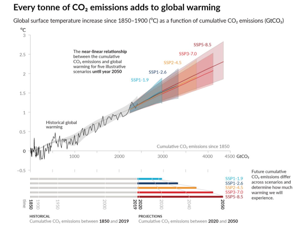
Global warming levels (GWLs) offer a relatively new way to look at and communicate future climate change. In this approach, the regional climate change response is shown relative to the average global warming (e.g., 0.5°C, 1.0°C, 1.5°C, 2.0°C) above a specified baseline period, typically pre-industrial (1850-1900).

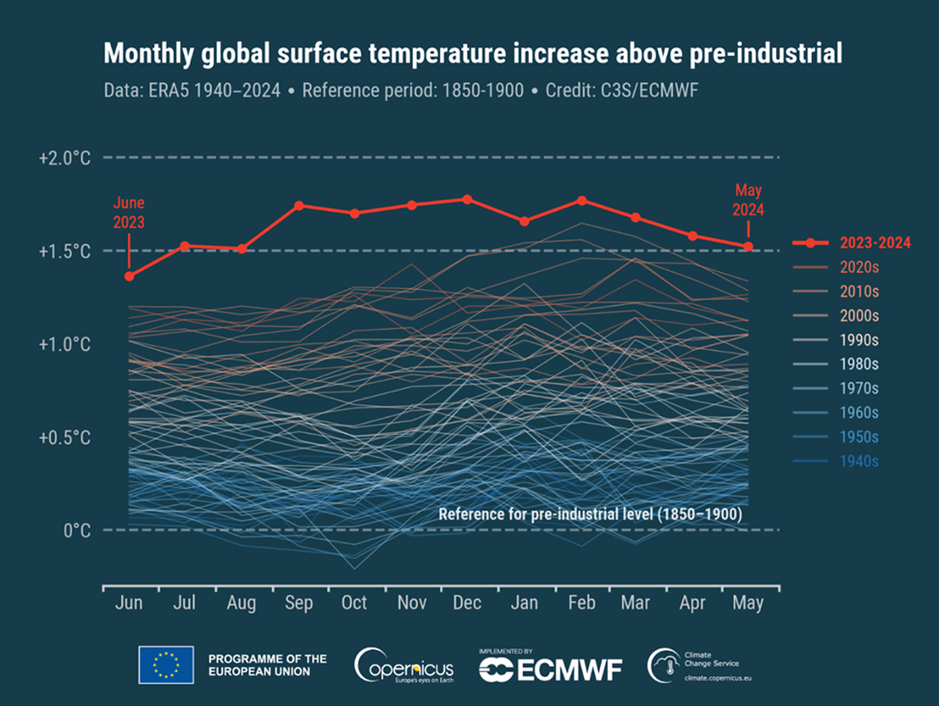
GWLs may already be familiar to some readers as they are often used in the media to track how current average temperatures compare to the pre-industrial baseline. For example, the Copernicus Climate Change Service regularly provides updates on monthly global temperature increases, with the most recent showing how observed climate has already exceeded the 1.5°C GWL in individual months (Figure 1). However, this type of analysis uses monthly averages for a particular year and is strongly influenced by natural climate variability.

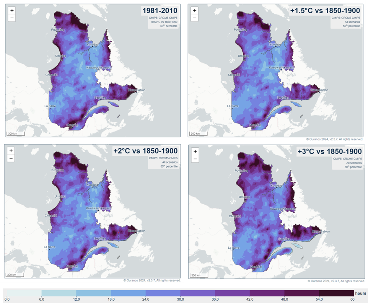
In the GWL approach described here, long-term average global mean temperature change (typically calculated over 20 or 30 years) is compared to regional climate changes averaged over the same period. Using longer averaging periods means that the global temperature change is less influenced by natural climate variability and exhibits a smoother trend over time thus making it easier to identify when a particular GWL is reached. This is the approach used in the Intergovernmental Panel on Climate Change (IPCC) Sixth Assessment Report to characterize projections of climate means and extremes, as well as climate impacts. It was also used  in the Pacific Climate Impacts Consortium’s Design Value Explorer, and to present projections of freezing rain in Ouranos’s Climate Portraits (Figure 2). On ClimateData.ca, GWLs are used in the Fire Weather Projections App and the Future Building Design Value Summaries.

Figure 1: Monthly global surface air temperature anomalies (°C) relative to pre-industrial (1850–1900) from January 1940 to May 2024, plotted as time series for all 12-month periods spanning June to May of the following year. The current GWL, defined based on a long-term mean, is approaching 1.5°C, and this figure illustrates how this level has already been exceeded in individual months. The June 2023 to May 2024 period is shown with a thick red line while all other years are represented using thin lines shaded according to the decade, from blue (1940s) to brick red (2020s). Data source: ERA5. Credit: C3S/ECMWF. [Source: Copernicus Climate Change Service]
Figure 2: Median number of hours of freezing rain (annual) for Québec for the CMIP5 ensemble, for current climate (1981-2010) and GWLs of 1.5°C, 2.0°C and 3.0°C, relative to pre-industrial (1850-1900) [Source: Ouranos Climate Portraits].

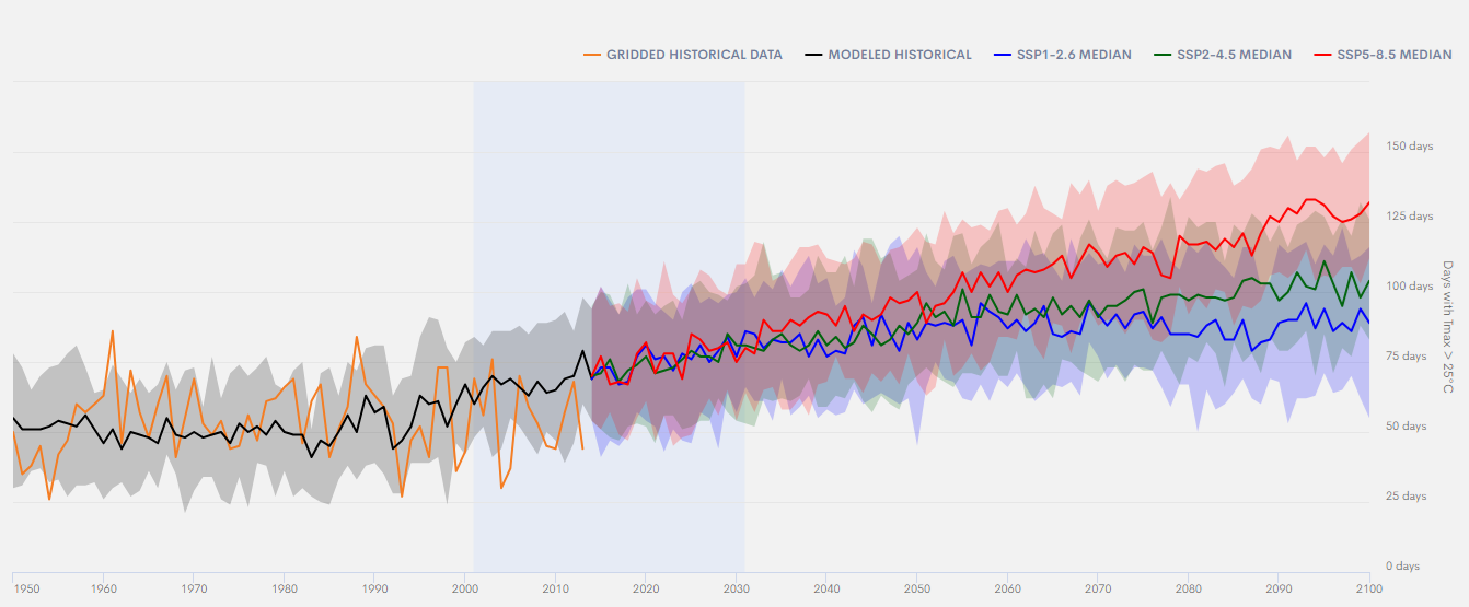
The main climate projections available on ClimateData.ca are shown by greenhouse gas emissions scenarios as time series plots and as maps which can be viewed for a particular time period. An example of this is shown in Figure 3, where a typical graph from ClimateData.ca shows the number of days with maximum temperature > 25°C over time for Regina, Saskatchewan (SK), according to each of three different emissions scenarios.

Figure 3: Example of the traditional approach used to present climate change projections, which shows the evolution of a particular climate variable by emissions scenario. Illustrated here are the number of days with maximum temperature >25°C for Regina, SK, according to three different emissions pathways (blue – SSP1-2.6; green – SSP2-4.5; red – SSP5-8.5) for the period 1950-2100.

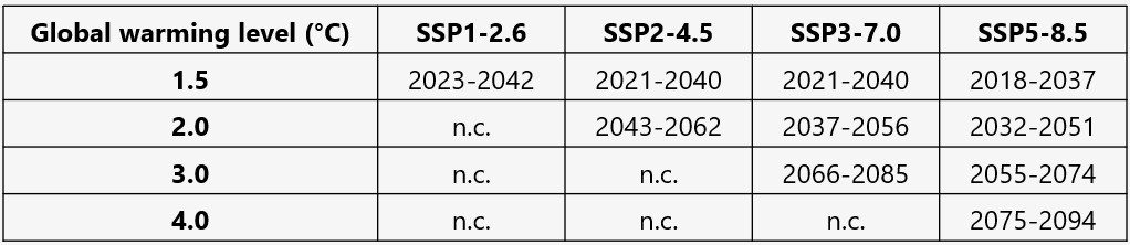
In the GWL approach, however, regional changes in a particular climate variable or index are shown in relation to the change in global average (mean) temperature rather than according to different emissions scenarios over time. This means that instead of illustrating what the range in magnitude of climate change is for the 2050s, for example, this approach instead shows what climate change is expected in Canada (or a subregion) when global warming reaches, say, 2°C. This type of analysis should be complemented, then, with information about when the particular GWL will be reached, which is dependent on future emissions.

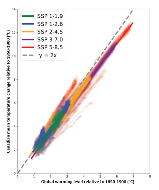
Figure 4 illustrates the relationship between annual average temperature changes for Canada and the globe, showing that Canada as a whole warms approximately twice as much (or as rapidly) as the global average. This means that for every 1°C increase in global average annual temperature, Canada’s average annual temperature increases by about 2°C. However, this approach does not provide information on the timing of when a particular level of global warming will occur. For more in depth information about the timing of GWLs, see More About Global Warming Levels.

Figure 4: Relationship between Canadian mean warming and global mean warming in CMIP6 simulations under five SSP scenarios. The dashed grey line (y=2x) corresponds to a warming rate for Canada that is twice the global rate [Source: Yongxiao Liang, Environment and Climate Change Canada].

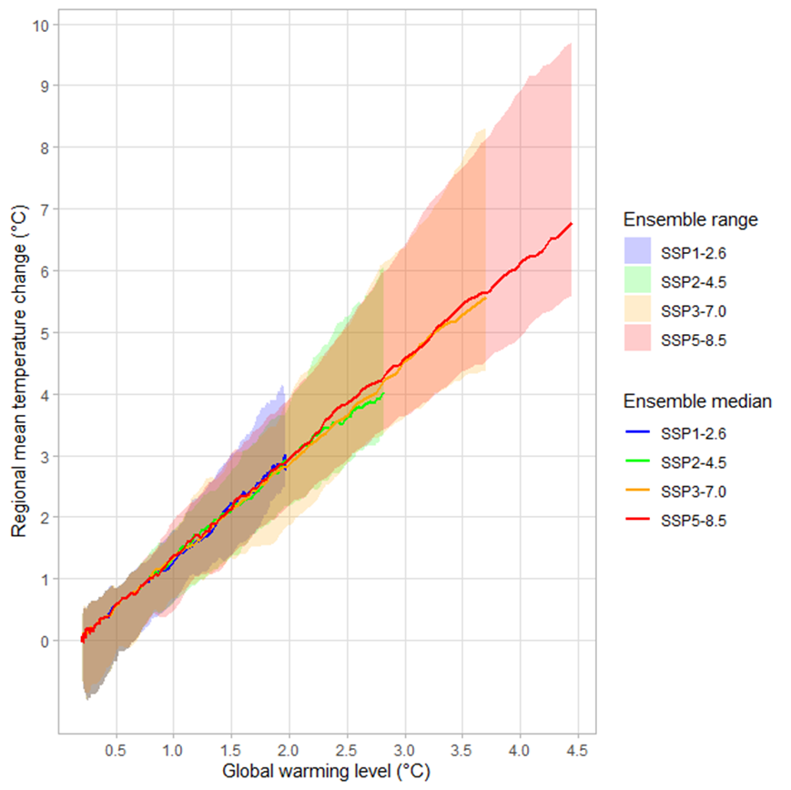
Regional changes in extreme temperatures and precipitation have been shown to scale robustly across emissions scenarios1 and these changes are almost linearly related to global average temperature change. As the global temperature rises, regional temperature extremes and heavy rainfall events tend to increase, a pattern that remains consistent across different emissions scenarios. This is also the case for other climate variables including mean temperature, which is illustrated in Figures 4 and 5. These figures illustrate that the regional warming at a given level of global warming is similar regardless of when that global warming occurs in a particular emissions scenario’s trajectory. Figure 4 compares annual mean temperature change at Canadian and global scales for five SSP emissions scenarios, while Figure 5 illustrates the almost identical regional-scale warming at different GWLs under four SSP emissions pathways used by the CMIP6 model ensemble. Research has demonstrated that  these findings are valid for a number of other climate variables,5,6,7 and also that the relationship between global warming level and regional changes in extremes may not necessarily be linear. For example, while the magnitude and frequency of less extreme regional heat events show a linear change with global warming, the frequency of rarer events, such as events with a 50-year return period, shows more of an exponential relationship with GWLs5. For example, at the global scale, such events are projected to become about 9, 14 and 40 times more frequent at GWLs of 1.5°C, 2.0°C and 4°C, respectively. In addition, the GWL approach does not tend to work well with variables which exhibit a substantial delay in their response to global temperature increase, e.g., sea level rise and glacial melt.

Figure 5: Example of a presentation of climate projections by levels of global warming. Here, mean temperature change for Saskatchewan is shown in relation to global average temperature change. This particular example uses a CMIP6 ensemble and the changes are calculated relative to the pre-industrial (1850-1900) reference period. Bold lines represent median values, and the shaded bands represent the range in the projections as defined by the 10th and 90th percentiles (SSP1-2.6 - blue; SSP2-4.5 - green; SSP3-7.0 - orange; SSP5-8.5 - red).

The regional spatial scale at which the relationship with GWLs is calculated also plays a role in determining the robustness of that relationship. In general, when changes to a particular climate variable or index are averaged over larger regions, there tends to be a clearer relationship with GWL because the averaging process reduces the influence of natural climate variability. Over smaller regions, the influence of natural climate variability is stronger and, as a result, the data appear noisier and the relationship between regional and global change is not necessarily as apparent. However, plotting global- versus regional-scale changes is a straightforward method  for identifying robust relationships.

What are the advantages of using GWLs?

Displaying future climate information using GWLs is becoming increasingly common, and there are several advantages to this approach:

  1. Direct Link to Global Temperature Goals of the Paris Agreement: Regional climate change can be more directly linked with climate policies that focus on keeping global warming below specific thresholds, in particular the Paris Agreement2. This Agreement aims to limit global warming to “well below 2°C” and to pursue efforts to limit warming to 1.5°C above pre-industrial levels. In the case of Canada, warming would be below 4°C from pre-industrial levels if global warming is kept below 2°C, or around 3.0°C if the 1.5°C limit is achieved. This approach makes it easier to see the regional consequences of achieving or missing global warming targets.

In the Summary for Policymakers of both the IPCC Fifth9 and Sixth4 Assessment Reports, it was shown that there is a clear linear relationship between cumulative CO2 emissions and the global climate response defined by  GWLs (Figure 6). By expressing the information in this way, it is easier to see exactly how different amounts of emissions correspond to global warming targets.

Figure 6: Near linear relationship between cumulative CO2 emissions and the increase in global surface temperature. For a full explanation of the figure see IPCC WG1 Figure SPM.10. [Source: Figure SPM.10 in IPCC, 2021: Summary for Policymakers. In: Climate Change 2021: The Physical Science Basis. Contribution of Working Group I to the Sixth Assessment Report of the Intergovernmental Panel on Climate Change [Masson-Delmotte, V., P. Zhai, A. Pirani, S.L. Connors, C. Péan, S. Berger, N. Caud, Y. Chen, L. Goldfarb, M.I. Gomis, M. Huang, K. Leitzell, E. Lonnoy, J.B.R. Matthews, T.K. Maycock, T. Waterfield, O. Yelekçi, R. Yu, and B. Zhou (eds.)]. Cambridge University Press, Cambridge, UK and New York, NY,USA, pp. 3−32, doi: 10.1017/9781009157896.001]4 ]
  1. Reframing Uncertainty: The GWL approach shifts part of the uncertainty in regional climate projections from the magnitude of the change resulting from an uncertain amount of future global GHG emissions to the timing of specified levels of global average temperature increase. For example, Figure 5 illustrates that for a GWL of 1.5°C, the median warming for Saskatchewan is between 2.0°C and 2.5°C, and the uncertainty is represented in the range of timing for when this GWL will be reached. Based on multiple lines of evidence, a GWL of 1.5°C is projected to occur between 2018-2037 (SSP5-8.5) and 2023-2042 (SSP1-2.6) (see Table 1). The timing of GWLs is discussed in More About Global Warming Levels.


Table 1: Summary of results for 20-year averaged change in global surface temperature (GWL) based on multiple lines of evidence. The first 20-year period during which the average global surface temperature change (°C) exceeds the specified global warming level relative to the pre-industrial period (1850-1900) is shown. An “n.c.” indicates that the global warming level is not crossed during the period 2021-2100. [Source: Adapted from IPCC Cross-Section box TS.1 Table 18].
  1. Ease of Communication: The GWL-based approach can simplify the communication of complex information to users, particularly those who are considering future climate projections from a risk-based perspective. For example, linking regional-scale changes to projected global warming means that the regional consequences of global-scale changes can be more readily understood. Since the projected changes in global average temperature are generally much smaller than the expected changes in temperature averages and extremes at the regional and country level, linking them in this way helps elucidate the expected regional consequences of global temperature targets.


  1. Comprehensive Information in GWL Graphics: Plots typical of the GWL approach contain valuable information, such as:
    1. The regional-scale response of the climate variable/index in question at different levels of global average temperature change (which, in turn, can be related to greenhouse gas emissions);
    2. An empirical assessment of the relationship between regional and global change for the climate variable/index in question – thus allowing easy identification of strong quantitative relationships at different spatial scales;
    3. The range of model and scenario response around the GWLs.

Limitations of the GWL approach

While the GWL approach is useful for linking regional and global climate change, it does have some limitations when it comes to informing adaptation. More detailed information is provided about these in More About Global Warming Levels.

The main limitations are:

  1. Multiple futures: Using the GWL approach does not eliminate the need to consider multiple futures that may occur under different emissions trajectories. Instead of choosing a range of plausible emissions scenarios, it becomes necessary to choose a range of relevant GWLs for a time period of interest.
  2. GWL selection: Selecting which GWLs to use may not be straightforward.
  3. Uncertainty in timing: There remains considerable uncertainty in the timing of when particular GWLs are reached, both between different scenarios and for individual scenarios.

In short, expressing climate projections using the GWL approach makes it easier to relate global warming targets to regional impacts and is a useful complement to the emissions scenario approach for presenting climate change projections.

References

  1. Seneviratne SI, Donat MG, Pitman AJ, Knutti R, Wilby RL (2016): Allowable CO2 emissions based on regional and impact-related climate targets. Nature 529: 477-483. Doi: 10.1038/nature16542
  2. UNFCCC, 2016: Decision 1/CP.21: Adoption of the Paris Agreement. In: Report of the Conference of the Parties on its twenty-first session, held in Paris from 30 November to 13 December 2015. Addendum: Part two: Action taken by the Conference of the Parties at its twenty-first session. FCCC/CP/2015/10/Add.1, United Nations Framework Convention on Climate Change (UNFCCC), pp. 1–36, https://unfccc.int/documents/9097.
  3. Cannon AJ, Jeong DI, Zhang X, Zwiers FW (2020): Climate-resilient buildings and core public infrastructure: An assessment of the impact of climate change on climatic design data in Canada. Government of Canada, Ottawa, ON, 106 p.
  4. IPCC WG1 SPM (2021): Summary for Policymakers. In: Climate Change 2021: The Physical Science Basis. Contribution of Working Group I to the Sixth Assessment Report of the Intergovernmental Panel on Climate Change [Masson-Delmotte V, Zhai P, Pirani A, Connors SL, Péan C, Berger S, Caud N, Chen Y, Goldfarb L, Gomis MI, Huang M, Leitzell K, Lonnoy E, Matthews JBR, Maycock TK, Waterfield T, Yelekçi O, Yu R, Zhou B (eds.)]. Cambridge University Press, Cambridge, UK and New York, NY,USA, pp. 3−32, doi: 10.1017/9781009157896.001 .]
  5. Tebaldi C, Adalgeirsdóttir G, Drijfhout S, Dunne J, Edwards TL, Fischer E, Fyfe JC, Jones RG, Kopp RE, Koven C, Krinner G, Otto F, Ruane AC, Seneviratne SI, Sillman J, Szopa S, Zanis P (2023): The hazard components of representative key risks. The physical climate perspective. Climate Risk Management 40: 100516. https://doi.org/10.1016/j.crm.2023.100516.
  6. Schwingshackl C, Sillman J, Vicedo-Cabrera A, Sandstad M, Aunan K (2021): Heat stress indicators in CMIP6: Estimating future trends and exceedances in impact-relevant thresholds. Earth’s Future 9: e2020EF001885. https://doi.org/10.1029/2020EF001885.
  7. Sobie SR, Zwiers FW & Curry CL (2021): Climate Model Projections for Canada: A Comparison of CMIP5 and CMIP6. Atmosphere-Ocean 59:4-5, 269-284. https://doi.org/10.1080/07055900.2021.2011103.
  8. Arias, P.A., N. Bellouin, E. Coppola, R.G. Jones, G. Krinner, J. Marotzke, V. Naik, M.D. Palmer, G.-K. Plattner, J. Rogelj, M. Rojas, J. Sillmann, T. Storelvmo, P.W. Thorne, B. Trewin, K. Achuta Rao, B. Adhikary, R.P. Allan, K. Armour, G. Bala, R. Barimalala, S. Berger, J.G. Canadell, C. Cassou, A. Cherchi, W. Collins, W.D. Collins, S.L. Connors, S. Corti, F. Cruz, F.J. Dentener, C. Dereczynski, A. Di Luca, A. Diongue Niang, F.J. Doblas-Reyes, A. Dosio, H. Douville, F. Engelbrecht, V. Eyring, E. Fischer, P. Forster, B. Fox-Kemper, J.S. Fuglestvedt, J.C. Fyfe, N.P. Gillett, L. Goldfarb, I. Gorodetskaya, J.M. Gutierrez, R. Hamdi, E. Hawkins, H.T. Hewitt, P. Hope, A.S. Islam, C. Jones, D.S. Kaufman, R.E. Kopp, Y. Kosaka, J. Kossin, S. Krakovska, J.-Y. Lee, J. Li, T. Mauritsen, T.K. Maycock, M. Meinshausen, S.-K. Min, P.M.S. Monteiro, T. Ngo-Duc, F. Otto, I. Pinto, A. Pirani, K. Raghavan, R. Ranasinghe, A.C. Ruane, L. Ruiz, J.-B. Sallée, B.H. Samset, S. Sathyendranath, S.I. Seneviratne, A.A. Sörensson, S. Szopa, I. Takayabu, A.-M. Tréguier, B. van den Hurk, R. Vautard, K. von Schuckmann, S. Zaehle, X. Zhang, and K. Zickfeld (2021): Technical Summary. In Climate Change 2021: The Physical Science Basis. Contribution of Working Group I to the Sixth Assessment Report of the Intergovernmental Panel on Climate Change [Masson-Delmotte, V., P. Zhai, A. Pirani, S.L. Connors, C. Péan, S. Berger, N. Caud, Y. Chen, L. Goldfarb, M.I. Gomis, M. Huang, K. Leitzell, E. Lonnoy, J.B.R. Matthews, T.K. Maycock, T. Waterfield, O. Yelekçi, R. Yu, and B. Zhou (eds.)]. Cambridge University Press, Cambridge, United Kingdom and New York, NY, USA, pp. 33−144. doi: 10.1017/9781009157896.002.
  9. IPCC (2013): Summary for Policymakers. In: Climate Change 2013: The Physical Science Basis. Contribution of Working Group I to the Fifth Assessment Report of the Intergovernmental Panel on Climate Change [Stocker, T.F., D. Qin, G.-K. Plattner, M. Tignor, S.K. Allen, J. Boschung, A. Nauels, Y. Xia, V. Bex and P.M. Midgley (eds.)]. Cambridge University Press, Cambridge, United Kingdom and New York, NY, USA.