More About Global Warming Levels

Global warming levels (GWLs) offer a relatively new way of presenting and communicating climate change projections. This approach links regional climate changes to specific levels of global warming and can be used to explore future regional climates associated with global climate policy goals, such as those of the Paris Agreement. Linking regional and global climate projections in this way characterizes the regional implications of projected global average temperature change and global climate change targets.

Key Messages

  • GWLs can be used to explore and compare regional changes in climate at specified levels of global warming, including the limits on global temperature increase committed to in the Paris Agreement.
  • The GWL approach shifts the uncertainty in regional climate projections from the magnitude of change associated with different emissions scenarios to the time when specific GWLs will be reached.
  • At more local scales, the influence of natural climate variability may make it difficult to identify robust relationships between regional climate and global temperature change.
  • The 1850-1900 pre-industrial baseline period is most commonly used (e.g., the IPCC Sixth Assessment Report and the Paris Agreement).  However, GWLs can be calculated using different baseline periods, so it is important to verify the baseline time period used to present data according to this approach.

What is the main difference between GWLs and the emissions scenario approach?

The primary distinction between a GWL approach and the more common emissions scenarios approach is in the articulation of regional climate projections. In the GWL approach, regional climate projections are expressed in relation to a specified increase in global average temperature above pre-industrial levels (or other baseline period), with no reference to when this increase in global average temperature could be reached. The emissions scenario approach presents climate projections by emissions scenario and, thus, indicates the trajectory of climate change against time for a given scenario. In this approach, the main uncertainty in regional climate projections is the magnitude of climate change for a specified emissions scenario. For the GWL approach, the main uncertainty in regional climate projections shifts to the time when specific GWLs will be reached. For some applications, e.g., for economic analyses, the lack of a continuous time series between now and a future time horizon may limit the utility of the GWL approach.

Which GWL should I use?

As with the choice of emissions scenario, selecting which GWL to use is context dependent. For example, if we are interested in examining the regional climate changes corresponding to levels that bracket the long-term temperature goal of the Paris Agreement2, i.e., to  keep “the increase in the global average temperature to well below 2°C above pre-industrial levels” and to pursue efforts “to limit the temperature increase to 1.5°C above pre-industrial levels”, we would choose GWLs of 1.5°C and 2.0°C above pre-industrial. If considering the projected global warming by the end of this century that aligns with current greenhouse gas reduction commitments, a GWL of 3.0°C above pre-industrial levels would be chosen7. If considering the possibility of a lack of adherence or reversal in current policies, or an underestimation of the sensitivity of global warming to emissions in climate models, a GWL of 4.0°C would be chosen. High GWLs such as 4.0°C are useful for exploring low probability, high impact outcomes, or for situations where a very low risk tolerance requires an abundance of caution.

For users working with specific time horizons, e.g., designing a building with a lifespan of 50 years, one will need to know which GWLs could be possible 50 years from now (e.g., 2075). Table 1 lists the estimated time at which different GWLs could be reached (based on 20-year averages from the ensemble of climate models used by Working Group 1 in the IPCC Sixth Assessment Report).  In this case, year 2075 falls roughly in the middle of one of the central estimates for approximately 3.0°C of warming under the SSP3-7.0 emissions scenario, and for approximately 3.5°C of warming under SSP5-8.5. For other emissions scenarios, the highest GWL ever attained is around 1.5°C for SSP1-2.6, and around 2°C for SSP2-4.5. Since average GWLs in excess of 2°C are not surpassed this century for these two emissions scenarios, GWLs to consider for 2075 would be between about 2°C and 3.5°C.  A user would choose these GWLs if they wanted to match the range of GWLs to the range of projected climate change for these four SSP-based emissions scenarios.

Table 1: Assessment results for 20-year averaged change in global surface temperature (GWL) based on multiple lines of evidence. GWLs are relative to the pre-industrial baseline period, 1850-1900. The first 20-year period during which the average global surface temperature change exceeds the specified level is shown. The entries give both the central estimate and, in parentheses, the very likely range (5-95%). An “n.c.” indicates that the GWL is not reached during the period 2021-2100.[Source:  Adapted from IPCC Cross-Section box TS.1 Table 15]

GWLs and baseline periods

It is important to note that GWLs are expressed as changes (or anomalies) calculated with respect to a baseline reference period. While the Paris Agreement2 refers to the pre-industrial period and IPCC uses specific definitions of (near) pre-industrial periods, most commonly 1850-1900, different baseline periods may be used to define GWLs. For example, the Climate Resilient Buildings and Core Public Infrastructure Report (CRBCPI)3, which provides future building design values, uses 1986-2016 as its baseline. As such, care needs to be taken when comparing projections based on GWLs to ensure that baselines are understood. 

It is possible, however, to reconcile differences in baselines to standardize the definition of GWLs. For example, Figure 1 illustrates the timing of GWLs using two different baseline periods: the IPCC pre-industrial period (1850-1900; right axis) and the 1986-2016 baseline (left axis) used by CRBCPI. About 0.8°C of global warming has occurred between the IPCC and CRBCPI baselines.

Noting that the Paris Agreement target is to limit global warming to “well below 2°C above pre-industrial levels”, in this example we compare 1.5°C and 2°C above 1850-1900 with the corresponding GWLs using the CRBCPI baseline period. The 2°C GWL above the 1850-1900 level corresponds to about 1.2°C of warming if using the 1986-2016 baseline.  The  1.2°C of warming is projected to occur around 2040. Similarly, the more stringent 1.5°C target corresponds to a GWL of about 0.7°C using the CRBCPI baseline of 1986-2016 and is projected to occur in the mid-2020s.

The CRBCPI report and the Pacific Climate Impacts Consortium’s Design Value Explorer (DVE) tool provide information about future design values for a range of GWLs to supplement the information in the National Building Code of Canada. The Future Building Design Value summaries available on ClimateData.ca provide information for two GWLs, 1.5°C and 3.0°C, relevant for the design of short- to medium-term design service life components (10 to 30 years) and medium- to long-term design service life components (50+ years), respectively. These GWLs are relative to the 1986-2016 baseline and correspond to GWLs of 2.3°C and 3.8°C using the pre-industrial baseline.

Another baseline period that you may encounter is 1971-2000. About 0.5°C of global warming has occurred between the IPCC’s pre-industrial baseline reference period of 1850-1900 and 1971-2000. This means that a GWL of 2°C relative to 1971-2000 is roughly equivalent to a GWL of 2.5°C from the pre-industrial 1850-1900 baseline. Finally, while most of the time a GWL from pre-industrial means 1850-1900, there are different definitions of “pre-industrial”, so it is always important to check the actual time period that is being used to define the baseline.

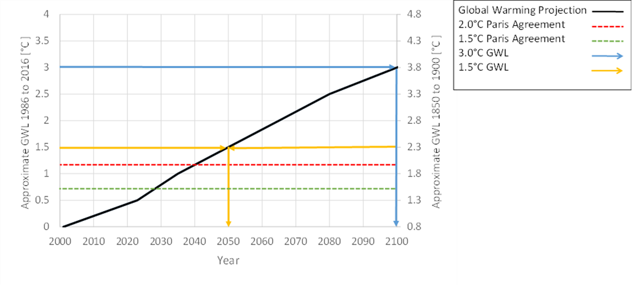
Figure 1: CRBCPI Simulated Global Warming Level evolution from the year 2000 to 2100. Superimposed are the 2050 and 2100 GWL of 1.5°C and GWL of 3.0°C, respectively, (baseline of 1986-2016; left axis), and the 1.5°C and 2°C GWLs (baseline of 1850-1900; right axis) used in this example to represent the Paris Agreement targets

What do you need to be aware of?

The GWL approach is based on robust relationships between regional climate changes and global average temperature shifts. This approach results from research into how regional temperature and precipitation extremes correlate with changes in global average temperature1. However, it is important to note that there are certain limitations that may affect the applicability of this approach across different climate variables, regions, and emissions pathways:

  1. The GWL approach is generally more successful at identifying robust relationships between global and regional scales for temperature-based indices, since they are directly related to changes in radiative forcing, which in turn are related to GHG emissions. Many temperature-based indices have been shown to scale linearly with global temperature change, e.g., number of frost days (minimum temperature < 0°C) and summer days (maximum temperature > 25°C).  In contrast, it is not always possible to identify robust relationships between the regional response of precipitation-based and other climate indices and global temperature change, and the strength of these relationships may vary by region4. In addition, the GWL approach does not tend to work well with variables that exhibit a substantial delay in their response to global temperature increase, e.g., sea level rise and glacial melt.  However, plotting global- versus regional-scale changes is a straightforward method for identifying robust relationships.
  2. For heavy precipitation events, although the ensemble-average response does scale robustly with global average temperature change, individual model projections may diverge strongly from this average response8. For precipitation, internal ‘natural’ climate variability plays a larger role at regional-to-local scales and precipitation extremes are much more spatially variable than temperature extremes.  Consequently, it can be more difficult to identify strong regional- to global-scale relationships for variables describing precipitation extremes. That said, however, for Canada as a whole, precipitation indices, including extremes, have been shown to scale robustly with GWLs.6
  3. Regional-scale relationships may also change over time, particularly if the response of a climate variable is strongly dependent on local forcing such as aerosols, land-use, and land cover change. For example, local aerosol forcing influences local precipitation amount, but becomes less important for larger regions. Also, projections of regional extreme precipitation may be different in emissions pathways which have the same, or similar, radiative forcing (e.g., SSP2-4.5 and RCP4.5) because the underlying assumptions for these emissions pathways may result in differences in local aerosol forcing.
  4. While robust relationships exist between the climate response of large regions when compared to the global scale, these relationships are expected to become less reliable for smaller regions, meaning that relationships between local and global scales are not always sufficiently strong to support the use of the GWL approach. For smaller regions, internal climate variability and local climate processes play a more significant role, increasing the ‘noise’ in the data and making it more difficult to see a distinct relationship between a climate variable and global average temperature change.
  5. Strong, quantitative (e.g., linear) relationships between climate variables and GWLs are less likely to be apparent under lower emissions scenarios, such as RCP2.6 or SSP1-2.6. This is due to a less strong climate signal when compared with the background noise of natural climate variability in projections using these emissions scenarios.

In short, expressing climate projections using the GWL approach makes it easier to relate global warming targets to regional impacts and is a useful complement to the emissions scenario approach for presenting climate change projections.

References

  1. Seneviratne SI, Donat MG, Pitman AJ, Knutti R, Wilby RL (2016): Allowable CO2 emissions based on regional and impact-related climate targets. Nature 529: 477-483. Doi: 10.1038/nature16542
  2. UNFCCC, 2016: Decision 1/CP.21: Adoption of the Paris Agreement. In: Report of the Conference of the Parties on its twenty-first session, held in Paris from 30 November to 13 December 2015. Addendum: Part two: Action taken by the Conference of the Parties at its twenty-first session. FCCC/CP/2015/10/Add.1, United Nations Framework Convention on Climate Change (UNFCCC), pp. 1–36, https://unfccc.int/documents/9097.
  3. Cannon AJ, Jeong DI, Zhang X, Zwiers FW (2020): Climate-resilient buildings and core public infrastructure: An assessment of the impact of climate change on climatic design data in Canada. Government of Canada, Ottawa, ON, 106 p.
  4. Tebaldi C, Adalgeirsdóttir G, Drijfhout S, Dunne J, Edwards TL, Fischer E, Fyfe JC, Jones RG, Kopp RE, Koven C, Krinner G, Otto F, Ruane AC, Seneviratne SI, Sillman J, Szopa S, Zanis P (2023): The hazard components of representative key risks. The physical climate perspective. Climate Risk Management 40: 100516. https://doi.org/10.1016/j.crm.2023.100516.
  5. Arias, P.A., N. Bellouin, E. Coppola, R.G. Jones, G. Krinner, J. Marotzke, V. Naik, M.D. Palmer, G.-K. Plattner, J. Rogelj, M. Rojas, J. Sillmann, T. Storelvmo, P.W. Thorne, B. Trewin, K. Achuta Rao, B. Adhikary, R.P. Allan, K. Armour, G. Bala, R. Barimalala, S. Berger, J.G. Canadell, C. Cassou, A. Cherchi, W. Collins, W.D. Collins, S.L. Connors, S. Corti, F. Cruz, F.J. Dentener, C. Dereczynski, A. Di Luca, A. Diongue Niang, F.J. Doblas-Reyes, A. Dosio, H. Douville, F. Engelbrecht, V. Eyring, E. Fischer, P. Forster, B. Fox-Kemper, J.S. Fuglestvedt, J.C. Fyfe, N.P. Gillett, L. Goldfarb, I. Gorodetskaya, J.M. Gutierrez, R. Hamdi, E. Hawkins, H.T. Hewitt, P. Hope, A.S. Islam, C. Jones, D.S. Kaufman, R.E. Kopp, Y. Kosaka, J. Kossin, S. Krakovska, J.-Y. Lee, J. Li, T. Mauritsen, T.K. Maycock, M. Meinshausen, S.-K. Min, P.M.S. Monteiro, T. Ngo-Duc, F. Otto, I. Pinto, A. Pirani, K. Raghavan, R. Ranasinghe, A.C. Ruane, L. Ruiz, J.-B. Sallée, B.H. Samset, S. Sathyendranath, S.I. Seneviratne, A.A. Sörensson, S. Szopa, I. Takayabu, A.-M. Tréguier, B. van den Hurk, R. Vautard, K. von Schuckmann, S. Zaehle, X. Zhang, and K. Zickfeld, 2021: Technical Summary. In Climate Change 2021: The Physical Science Basis. Contribution of Working Group I to the Sixth Assessment Report of the Intergovernmental Panel on Climate Change [Masson-Delmotte, V., P. Zhai, A. Pirani, S.L. Connors, C. Péan, S. Berger, N. Caud, Y. Chen, L. Goldfarb, M.I. Gomis, M. Huang, K. Leitzell, E. Lonnoy, J.B.R. Matthews, T.K. Maycock, T. Waterfield, O. Yelekçi, R. Yu, and B. Zhou (eds.)]. Cambridge University Press, Cambridge, United Kingdom and New York, NY, USA, pp. 33−144. doi: 10.1017/9781009157896.002.
  6. Sobie SR, Zwiers FW & Curry CL (2021): Climate Model Projections for Canada: A Comparison of CMIP5 and CMIP6. Atmosphere-Ocean 59:4-5, 269-284. https://doi.org/10.1080/07055900.2021.2011103.
  7. United Nations Environment Programme (2023): Emissions Gap Report 2023: Broken Record – Temperatures hit new highs, yet world fails to cut emissions (again). Nairobi. https://doi.org/10.59117/20.500.11822/43922.
  8. Evin G, Ribes A, Corre L (2024): Assessing CMIP6 uncertainties at global warming levels. Climate Dynamics. https://doi.org/10.1007/s00382-024-07323-x