Understanding climate extremes: Return Periods and Return Levels

Learn about extreme events, return periods and return levels, and the associated data available on ClimateData.ca.

Module

Understanding Future Projections

Format

Article

Time to completion

15 minutes

Key Messages


  • Extreme events are often described using two concepts: return periods and return levels.
    • Return periods quantify the average frequency of recurrence of extreme events. They are an estimate of how often, on average, an extreme event of a certain magnitude is expected to occur.
    • Return levels quantify the magnitude of an event associated with a particular return period.
  • Return periods and return levels do not indicate that an event will occur in a specific time period. For example, a 1-in-50-year event has, on average, a 2% chance of occurring in any given year, meaning that multiple or even no 1-in-50-year events may happen within a specific 50-year period.
  • ClimateData.ca offers return level data for several different return periods for three variables: annual maximum daily temperature, annual minimum temperature and annual maximum one-day precipitation

Introduction


This article provides an overview of the return level data available on ClimateData.ca and the related concepts needed to interpret it. Return levels describe the magnitude of an event with a specified occurrence frequency or return period. This article also addresses common misconceptions about return levels and return periods.

How are extreme events described?


Extreme weather events, such as extreme heatwaves and heavy rainstorms, are intense phenomena that deviate from normal weather conditions. Extreme events are often described in terms of their frequency (return period) and magnitude (return level). Both metrics can be used to assess risks and plan for extreme weather events.

Return period and return level data have numerous applications, including informing processes such as bridge and dam design, water resource management, supporting catastrophe modelling, and risk assessments. One way that these data are commonly presented is as an Intensity-Duration-Frequency (IDF) curve. IDF curves describe rainfall magnitudes of different durations corresponding to certain frequencies of occurrence thus aiding in the design of stormwater systems and flood control measures.

What are return periods?

A return period is the average time interval between event occurrences of a specific magnitude.  An event with an x-year return period is commonly described as “1-in-x-year event” or an “x-year event”, where x is the estimated number of years between events. Longer return period events (e.g., 1-in-50-year) are more extreme than shorter return period events (e.g., 1-in-20- or 1-in-10-year), see Figure 1.

An event with a specific return period is not guaranteed to occur exactly once within that timeframe; it may occur more frequently, or not at all, as seen in Figure 1. For example, a “1-in-50-year flood” refers to a flood event with a return period of 50 years. This means that such an event is expected to occur once every 50 years or, described another way, has about a 2% chance of occurring in any given year during this period.

Figure 1: A depiction of the potential occurrences of 1-in-50-year and 1-in-20-year return period events across a 200-year period. This visualization demonstrates that an event with a specific return period is not guaranteed to occur exactly once within that timeframe; it may occur more frequently, or not at all. The magnitude of each event is represented by the icon size, with longer return period events (e.g., 1-in-50-year) corresponding to a more extreme event than shorter return period events (e.g., 1-in-20- or 1-in-10-year).

How can climate change impact return periods?


The frequency of events of a particular magnitude may change over time because of climate change (Figure 2). For example, a maximum precipitation event with a 1-in-20-year return period (5% probability of occurrence) may become closer to a 1-in-10-year event (10% probability of occurrence) in the future.

Figure 2: Example showing how climate change may impact the frequency of an event with a specific return level. During the historical period (shown on top), an event of this magnitude has a 1-in-20-year return period. In a future climate (shown on the bottom), an event of this magnitude may become more frequent with the return period shortening from 1-in-20 years to approximately 1-in-10 years on average. Here a single emissions scenario is used for illustration, but best practice is to look at a range of different emissions scenarios to assess the range of possible future return levels.

What are return levels?


A return level is the magnitude of an event associated with a specific return period. For example, if a maximum daily temperature with a 1-in-50-year return period has a return level of 45°C, it means a daily maximum temperature of 45°C or higher is expected to occur, on average, once every 50 years. In this case, in any given year, the probability of reaching or exceeding 45°C is about 1-in-50 or 2%.

At a given location, longer return period events (e.g., 1-in-50-year) correspond to more extreme events, than shorter return period events (e.g., 1-in-20 or 1-in-10 year).


How can climate change impact return levels?


Climate change means that the magnitude of events of a particular frequency may change over time (Figure 3). For example, a one-day maximum precipitation event with a 1-in-20-year return period (5% probability of occurrence) may have been a 40mm event in the past climate but may become closer to a 55mm event in the future climate.

Figure 3: Example showing how climate change may impact the magnitude of 1-in-20-year events. The magnitude of each event is represented by the icon size. During the historical period (shown on top), a 1-in-20-year storm has a particular magnitude. In a future climate (shown on the bottom), an event of this frequency may become larger in magnitude. Here a single emissions scenario is used for illustration, but best practice is to look at a range of different emissions scenarios to assess the range of possible future return levels

Common misconceptions


Misconception 1:

An event with a particular return period will happen exactly once in that period. For example, a 1-in-50-year extreme event will only happen once over a fixed 50-year period.

Fact:

A 1-in-50-year extreme event has about a 2% probability of occurring annually. This means that it is possible to experience multiple 1-in-50-year extreme events within a given 50-year period, or none at all. In fact, there is about a 37% chance that a 50-yr event happens exactly once in a 50-year period and about 26.5% probability for more than one to occur. Figure 2 illustrates a plausible example of how 1-in-50-year return period events could play out.


Misconception 2:

An event with a particular return period will be the most severe event in that period. For example, a 1-in-50-year extreme event is the most severe event that will happen in 50 years.          

Fact:

A 1-in-50-year extreme event, and its associated magnitude (its return level), has about a 2% chance of occurring annually. This does not mean, however, that a higher magnitude event cannot also occur within 50 years.

How to find and interpret the return level data on ClimateData.ca


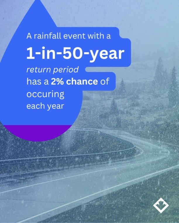
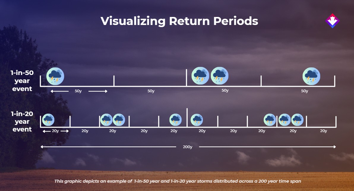
ClimateData.ca provides return level projections for 1-in-5-, 1-in-10-, 1-in-20-year, 1-in-30-year and 1-in-50-year events and various emissions scenarios over different periods, allowing users to explore potential extremes in future climates. The return levels of the following variables are available on ClimateData.ca:

  • Annual Maximum Temperature: This represents the highest daily maximum temperature of the year.
  • Annual Minimum Temperature: This represents the lowest daily minimum temperature of the year.
  • Annual Maximum 1-day Precipitation: This represents the highest 1-day precipitation total of the year.

To explore return level projections on ClimateData.ca, navigate to the map, select the desired return level, variable, emissions scenario and time period. The resulting map will be the median (50th percentile) return level from the climate model ensemble.

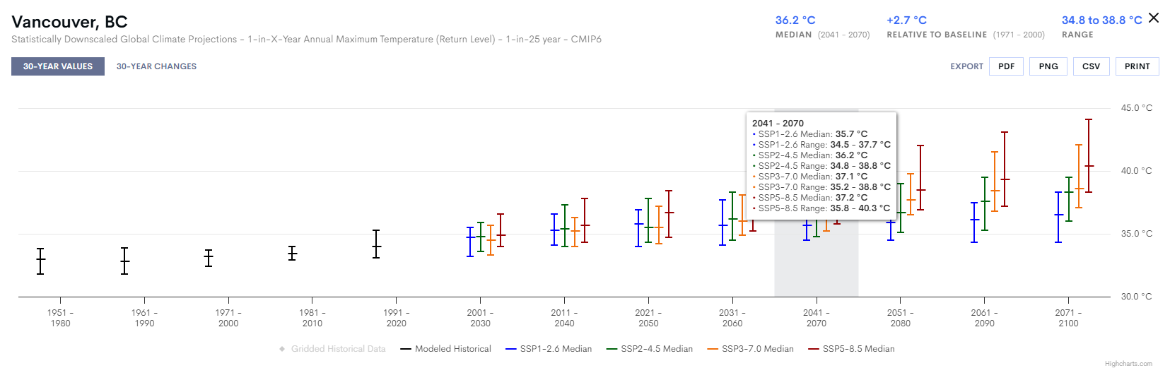
To see how return levels are projected to evolve over the century, either search for a location using the search bar, or zoom in and select a grid cell. A summary box will appear with the median and range of projections for that time period, as well as the projected difference relative to the 1971-2000 period. Clicking “See details” will bring up a plot as seen in Figure 4.

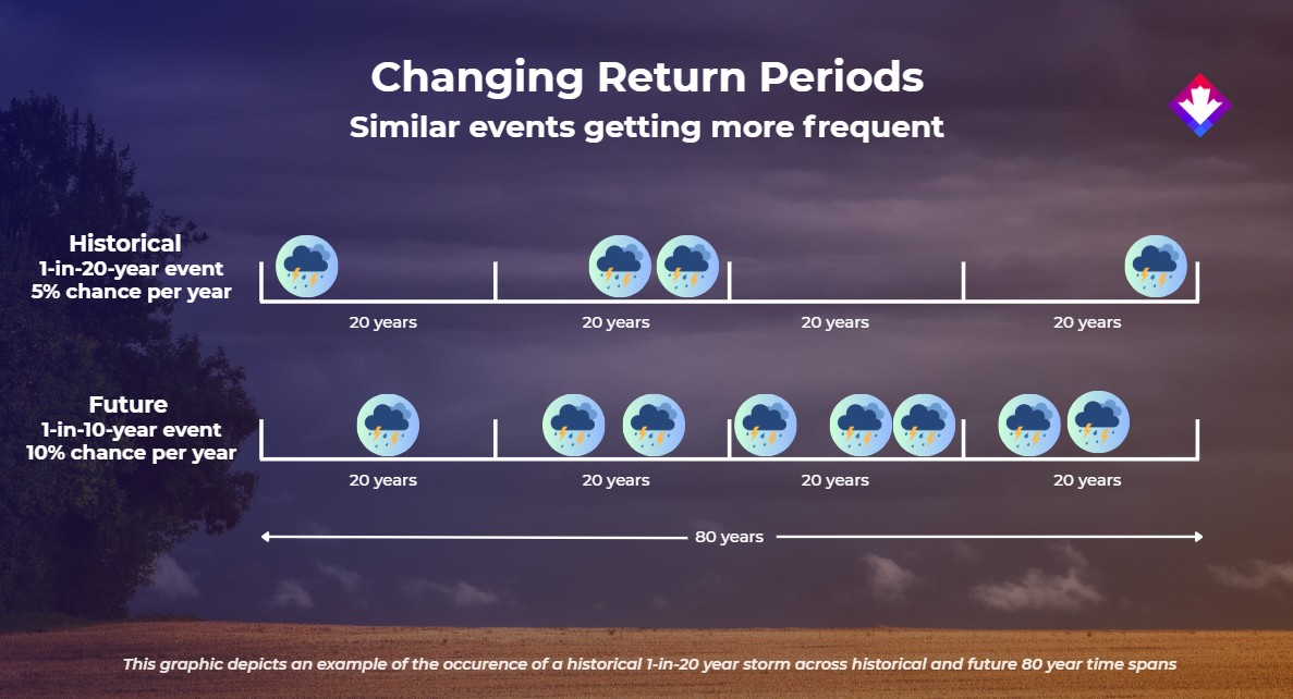
The time series plots include four emissions scenarios and hovering over the plot will bring up a tooltip with data for each scenario. For example, in Figure 4 the median value of the climate model ensemble indicates that under the SSP2-4.5 emissions scenario there is, on average, a 1-in-25 chance per year that the maximum daily temperature will reach or exceed 36.2°C in the 2041-2070 timeframe.

Figure 4: Example of a return level time series graph on ClimateData.ca.

ClimateData.ca provides the median (50th percentile) return level and range (10th and 90th percentiles). It is important to explore a range of emissions scenarios and percentiles to gain a more comprehensive understanding of potential future climate extremes. For example, by considering the 10th and 90th percentile values for a given emissions scenario, users can assess a wider range of change from the climate model ensemble (which helps address climate model uncertainty). Similarly, exploring different SSPs allows for an assessment of how various socio-economic and global policy choices might influence future climate (which helps address emissions scenario uncertainty).

Note that the plots displayed on ClimateData.ca represent average conditions over the grid-box of approximately 10 km x 6 km. Accordingly, the data does not necessarily reflect an individual point location within each grid cell – particularly in areas with varying topography. In such cases, the change in return level from past to future (accessed using the “delta” option on the map sidebar) may be applied to local station estimates of historical return levels.

Summary


Return periods and return levels are statistical metrics used to describe the frequency and magnitude of extreme weather events. These concepts are often expressed through terms such as a ‘100-year storm’ or a ‘1-in-100-year event’. Return period describes how often, on average, an event of certain magnitude is expected to occur, while return level describes the magnitude of an event associated with a particular return period. These metrics do not predict exactly when an event will occur but instead provide statistical information about extreme events during a particular timeframe. Return level projections for maximum daily temperature, minimum daily temperature, and maximum daily precipitation are now available on ClimateData.ca.

References


  1. Cook, N J (1986). Designers guide to wind loading of building structures. Part 1.
  2. Haan, C. T., Barfield, B. J., & Hayes, J. C. (1994). Hydrologic frequency analysis. Design hydrology and sedimentology for small catchments (pp. 5–36). Academic Press. https://doi.org/10.1016/B978-0-08-057164-5.50006-2
  3. Koliokosta, E. (2023). Return Periods in Assessing Climate Change Risks: Uses and Misuses. Environmental Sciences Proceedings, 26(1), Article 1. https://doi.org/10.3390/environsciproc2023026075